Equation of a straight line
All linear regression tutorials begin with the equation of a straight line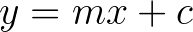
which is sometimes written as
or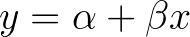
No matter how you write it the variables are the same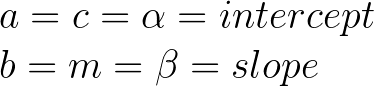
Linear regression
Linear regression is a concept where a line can be fit through a cloud of points. These point clouds are sometimes referred to as a scatterplot. When a line is passed through a scatterplot the points might not fall exactly on to the line, so we introduce the concept of ‘error’. The residual error is the vertical distance between each point and the line that passes through the scatterplot. Points that are close to the line have an error near zero, points above the line have an error that it positive and points below the line have an error that is negative.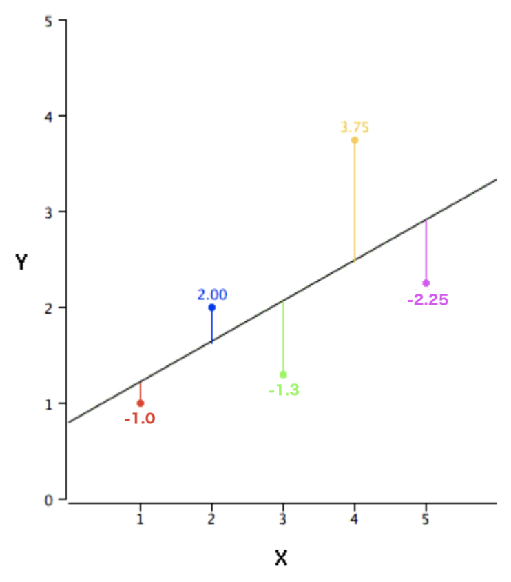
This concept of error can be introduced to the line equation so that given any x value the location of any point can be found in respect to the line. This gives us the linear regression equation.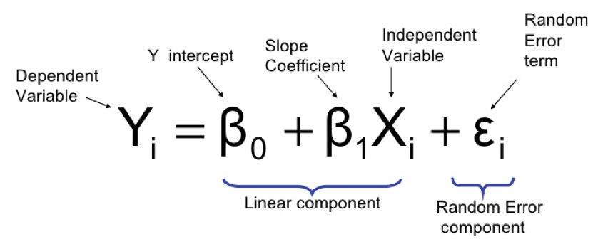
With linear regression the intercept and slope are wearing hats and are numbered but this is not any different than the traditional line equation.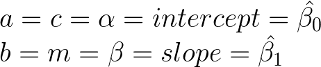
The hat just means it is an estimated parameter.
The best lines fit through a scatterplot in a way that it has the smallest error possible. This means the line should be as close as possible to the majority of the points. This can be solved by making the error as small as possible. The total error can be calculated by adding of the vertical distances of all the points to the line. Squaring the individual distances ensures the negative distances don’t cancel out the positive distances. This is called the Sum of Square Error (SSE).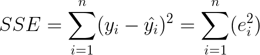
Error minimisation
By rearranging the linear regression equation so that the error is on its own, we can minimise the squared error to find a line that fits.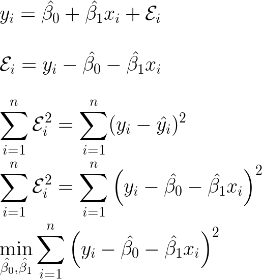
Rules of differentiation
There are some calculus rules you need to know before finding the derivatives. The chain, power, sum and difference rules. It is assumed you know these before moving on.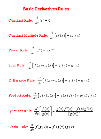
Derivation of ordinary least squares
In order the minimise the sum of the squared error, you must first calculate it’s partial derivitive with respect to its intercept and slope. To do this we use the power rule and the chain rule.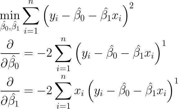
Setting the derivitives to zero
Univariate optimization involves taking the derivative and setting equal to 0. This minimization problem is solved by setting the partial derivatives equal to 0. That is, take the derivative of the first equation with respect to the intercept and set it equal to 0. We then do the same thing for the slope.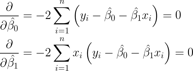
Solving for the intercept
The value for the intercept can be found by following a few rules. To do this you need to know the sum & difference rule: the derivative of a sum is the same as the sum of the derivatives.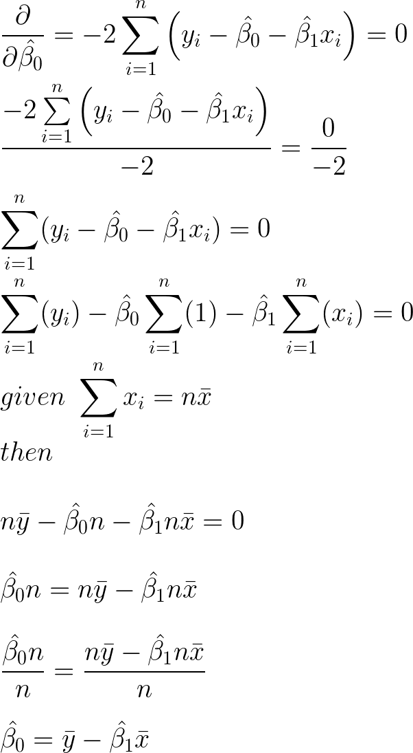
Solving for the slope
The solution for the intercept can be subsitituted in place. This takes the intercept out of the equation.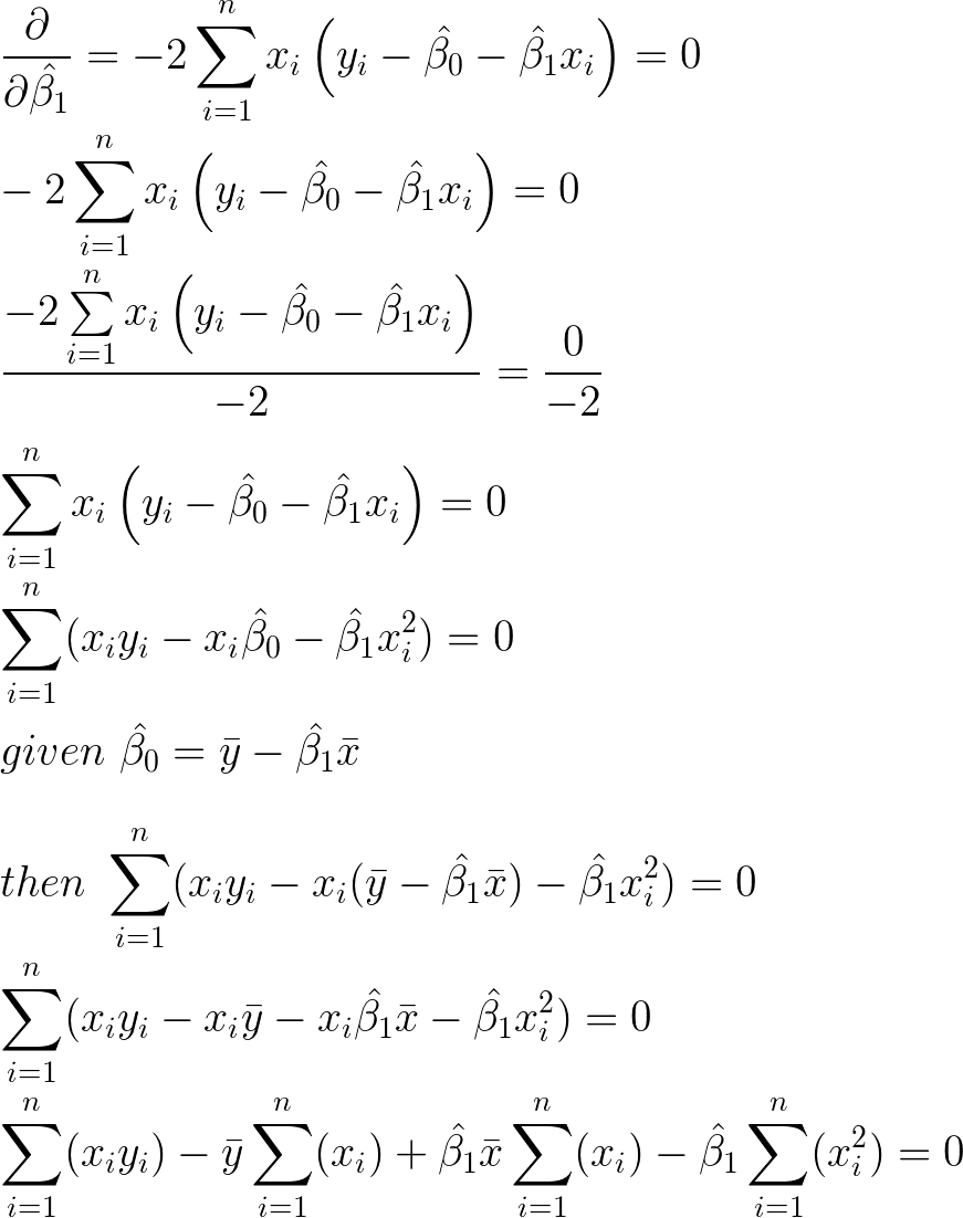
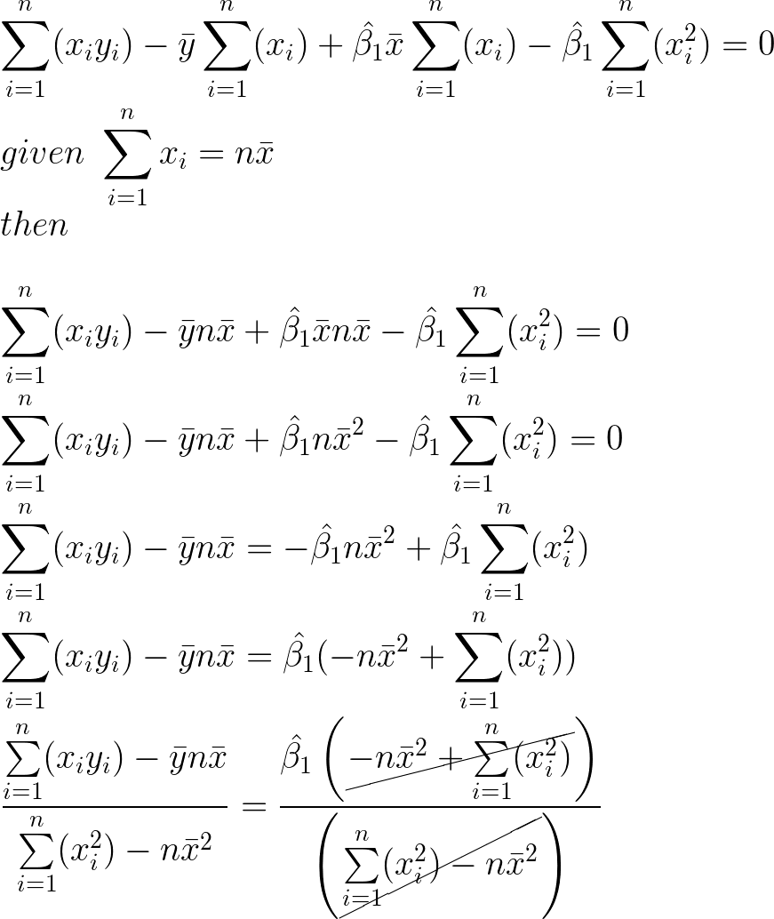
We now have a rudimentary slope, but it doesn’t match the equations in most textbooks.
Slope numerator refinement
We can easily derive the numerator of the equation to match what you would find in a textbook.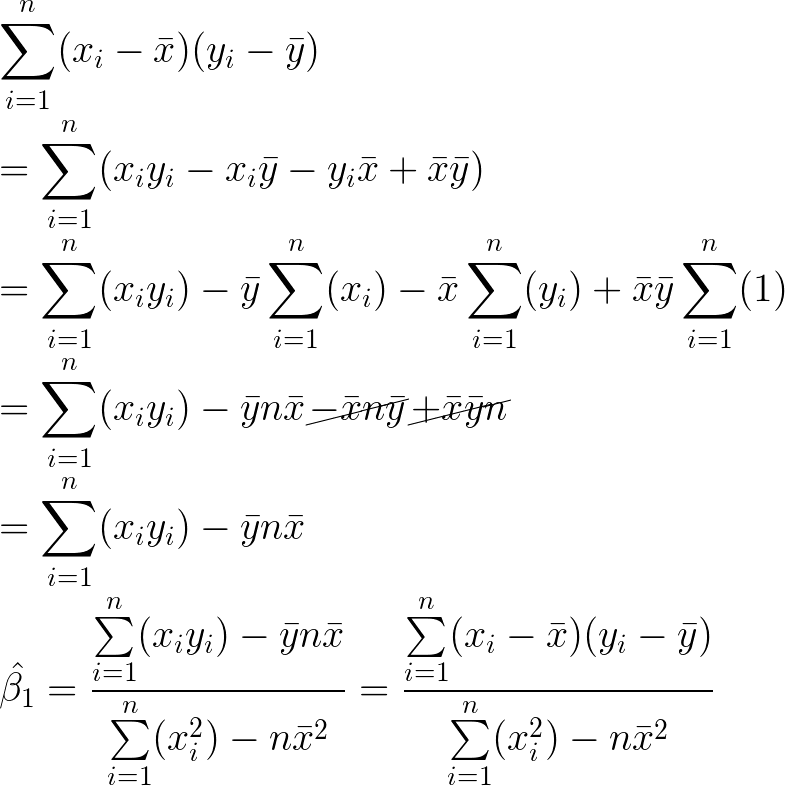
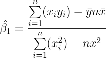
Slope denominator refinement
We can easily derive the denominator of the equation to match what you would find in a textbook.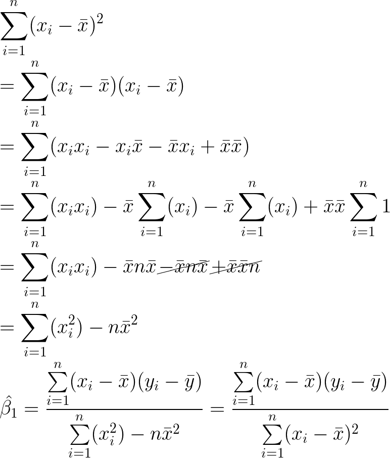
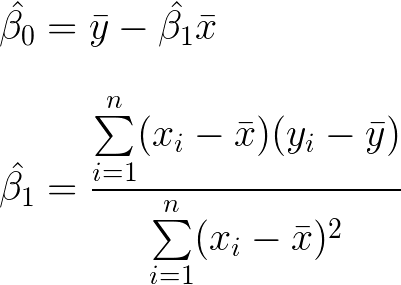
Ordinary least squares equations
The slope and y-intercept are now derived. The line of best fit can now easily be calculated.